I am currently taking Vizuara’s Kernel Engineering Workshop, taught by Dr. Raj Dandekar and Shubham Panchal. The course is about understanding how GPUs execute programs, then using that understanding to write faster kernels: the functions that run on the GPU. It starts with parallel execution, CUDA, and the memory hierarchy, then works through matrix multiplication, tensor cores, profiling, attention, and modern GPU programming tools. The lectures are paired with coding sessions so the explanations can be tested in working implementations.

This article grew out of the matrix multiplication work. Before moving on to tensor cores, we worked through seven versions of a kernel running on CUDA cores. Each version addressed a different source of overhead, from the way threads accessed global memory to the amount of work they kept in registers. By the seventh version the kernel was considerably more sophisticated, but there was still a gap to NVIDIA’s cuBLAS library. The instructor challenged us to see whether we could close it.

The course was already taking a substantial amount of my free time, so I explored the challenge without turning it into another lengthy assignment: I gave an LLM the existing kernels and a way to run experiments through my Modal account. The model did much of the implementation and profiling analysis, using Nsight Compute to inspect the results. My goals were to learn about optimizations beyond those covered in class and to share the findings with the course authors and other students.

The result was a small but repeatable win for one specific case, and a remaining gap everywhere else:

Size (n × n, FP32)	Best kernel	Time	cuBLAS	Speed vs. cuBLAS
1,024	k14, Stream-K (generic)	61.3 µs	64.6 µs	105.3%, faster in 15 of 15 rounds
2,048	k13f (size-specialized)	357.9 µs	341.3 µs	95.4% (generic k11: 93.9%)
4,096	k13f (size-specialized)	2,761.2 µs	2,661.1 µs	96.4% (generic k11: 95.2%)

All of these were measured on one NVIDIA H100 80GB with FP32 inputs and arithmetic and TF32 disabled for cuBLAS. This was an investigation of a particular FP32 workload, not a replacement for cuBLAS across arbitrary matrix sizes and precision modes. The rest of the article explains the operation, the seven kernels that established the starting point, and then each later change: the ones that helped, and the ones that looked promising in a profile but did not improve runtime.

n = 1,024n = 2,048n = 4,096cuBLAS = 100%

Show the data

Step	Change	n = 1,024	n = 2,048	n = 4,096
Course k7	course measurement	65%	—	—
k8	cp.async pipeline	89%	81%	81%
k9	register prefetch + transposed A	97%	83%	82%
k10	16×8 / 8×16 patches	92%	88%	90%
k11	hoisted address math	98%	94%	95%
k12	copies spread over k-steps	100%	96%	95%
k13	branch-free spread; size-specialised	98%	96%	96%
k14	Stream-K	107%	92%	94%
Confirm	15 alternating rounds	105.3%	95.4%	96.4%

The operation: GEMM and the precision of the comparison

The operation is matrix multiplication, usually discussed under the name GEMM: general matrix multiplication. For A with dimensions M × K and B with dimensions K × N, the product C is M × N, and each output element is the dot product of a row of A and a column of B:

C[m, n] = Σ_k A[m, k] × B[k, n]

The general BLAS routine computes C = αAB + βC; these experiments computed only AB, for square matrices whose sides are multiples of the tile size. NVIDIA’s matrix multiplication background guide covers the operation and its performance characteristics. That keeps the scope clear: a library routine also supports scaling, accumulation into an existing output, transposition, other layouts, and many shapes that these kernels did not attempt.

A straightforward implementation performs K multiply-adds for each of the M × N outputs, about 2MNK floating-point operations. The work is done by FFMA instructions: fused floating-point multiply-adds, where the multiplication and addition share a single final rounding. In throughput accounting, an FFMA still counts as two operations.

The inputs and arithmetic in the comparison were FP32: four-byte values with one sign bit, eight exponent bits, and 23 stored fraction bits. That is a stronger statement than saying the arrays had a 32-bit type, because a library can accept FP32 arrays and use a different internal arithmetic mode. TF32 (TensorFloat-32) is the important example on NVIDIA GPUs. It keeps FP32’s exponent range but uses fewer significand bits for the multiplication inputs on the tensor cores, which buys much higher throughput at the cost of different numerics (NVIDIA’s TF32 introduction). TF32 was disabled for the cuBLAS reference here, so both sides ran FFMA on the CUDA cores. A claim of beating cuBLAS without that qualification would leave out an essential part of the comparison.

The hardware model behind the changes

A CUDA kernel launches a grid of thread blocks. Threads within each block are grouped into warps of 32, and the GPU’s streaming multiprocessors (SMs) schedule those warps’ instructions. Global memory holds the matrices and is visible across the device. Shared memory belongs to a block and lets its threads reuse a loaded tile without asking global memory for the same data again. Registers hold per-thread values, including the partial sums, right next to the arithmetic. Moving data into a faster level does not remove the need to deliver it to the next one.

That gives three questions to ask of any version. Are neighboring lanes of a warp requesting data efficiently? Is each loaded value reused enough times to justify moving it? And is there enough independent work available while a load, or an instruction dependency, is waiting? The first seven kernels largely answered the first two. The later kernels were about the third: how reliably the layout could keep the arithmetic units supplied.

The foundation: the first seven kernels

The numbering follows my fork of the course repository. All seven were Python CUDA kernels written with Numba’s @cuda.jit and CuPy arrays: Python was the source language, and Numba compiled the device code for the GPU. Warp tiling was already in the course’s kernel 6, and kernel 7 tuned that design. Kernels 8 to 14 are my extension of the course work.

The important distinction in this part is between changing what each thread computes and changing where its operands live.

Kernel 1: a correct baseline

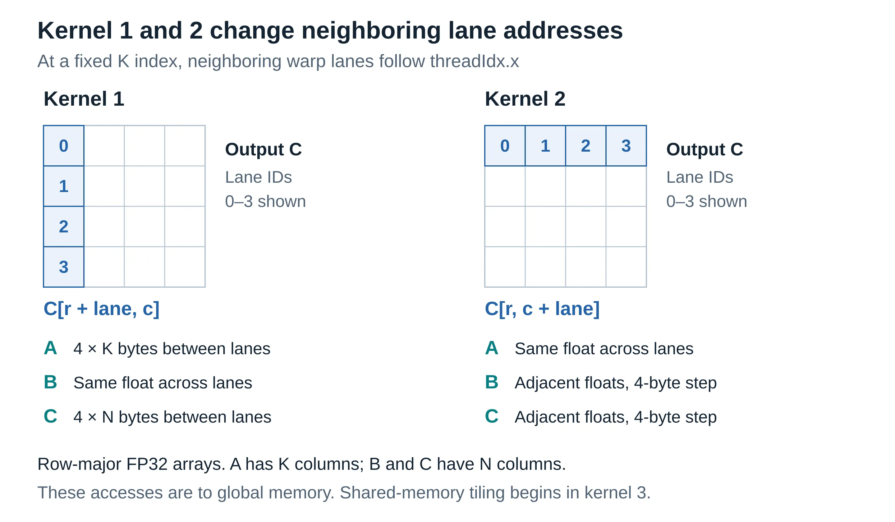
Kernel 1 assigned one output element to each thread. That is an easy starting point for checking correctness, but its mapping sent neighboring lanes of a warp down different output rows. The arrays are row-major, so adjacent columns sit next to each other in memory and adjacent rows do not. Holding k fixed and looking across one warp: every lane requested the same B value, while the A reads and C writes were each separated by a full row stride. Kernel 1 read its operands directly from global memory, with no shared-memory staging.

That mattered before any attempt to pipeline the computation. A GPU moves memory in transactions, not by charging only for the bytes the program uses, and scattered lane requests can need many more transactions than a contiguous group.

Kernel 2: make neighboring lanes match the layout

Kernel 2 swapped the mapping so neighboring lanes worked across output columns. For a fixed row and k, every lane needed the same A[m, k], each needed a neighboring B[k, n], and the output writes advanced across columns. The arithmetic was unchanged; the improvement came entirely from how the warp requested its data.

This is coalescing: how a warp’s memory requests can be combined. It does not guarantee one physical transaction per access, since alignment, access width, and the exact addresses still matter. The useful change was that neighboring lanes no longer made row-strided A requests and C writes.

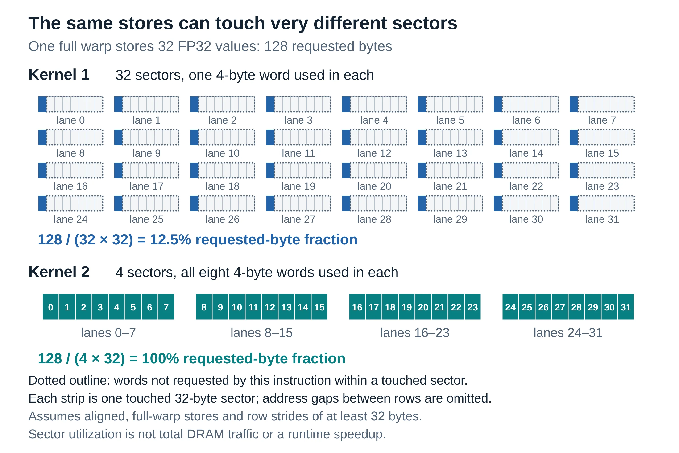
For one aligned, full-warp FP32 store, the difference is concrete. Kernel 1 wrote 32 four-byte values to 32 different rows. In the notebook’s example the C row stride is 800 × 4 = 3,200 bytes, so those writes touched 32 separate 32-byte sectors, and the 128 bytes written filled one eighth of them. Kernel 2 wrote the same 128 bytes across adjacent columns, filling four aligned sectors completely.

Kernel 3: reuse tiles in shared memory

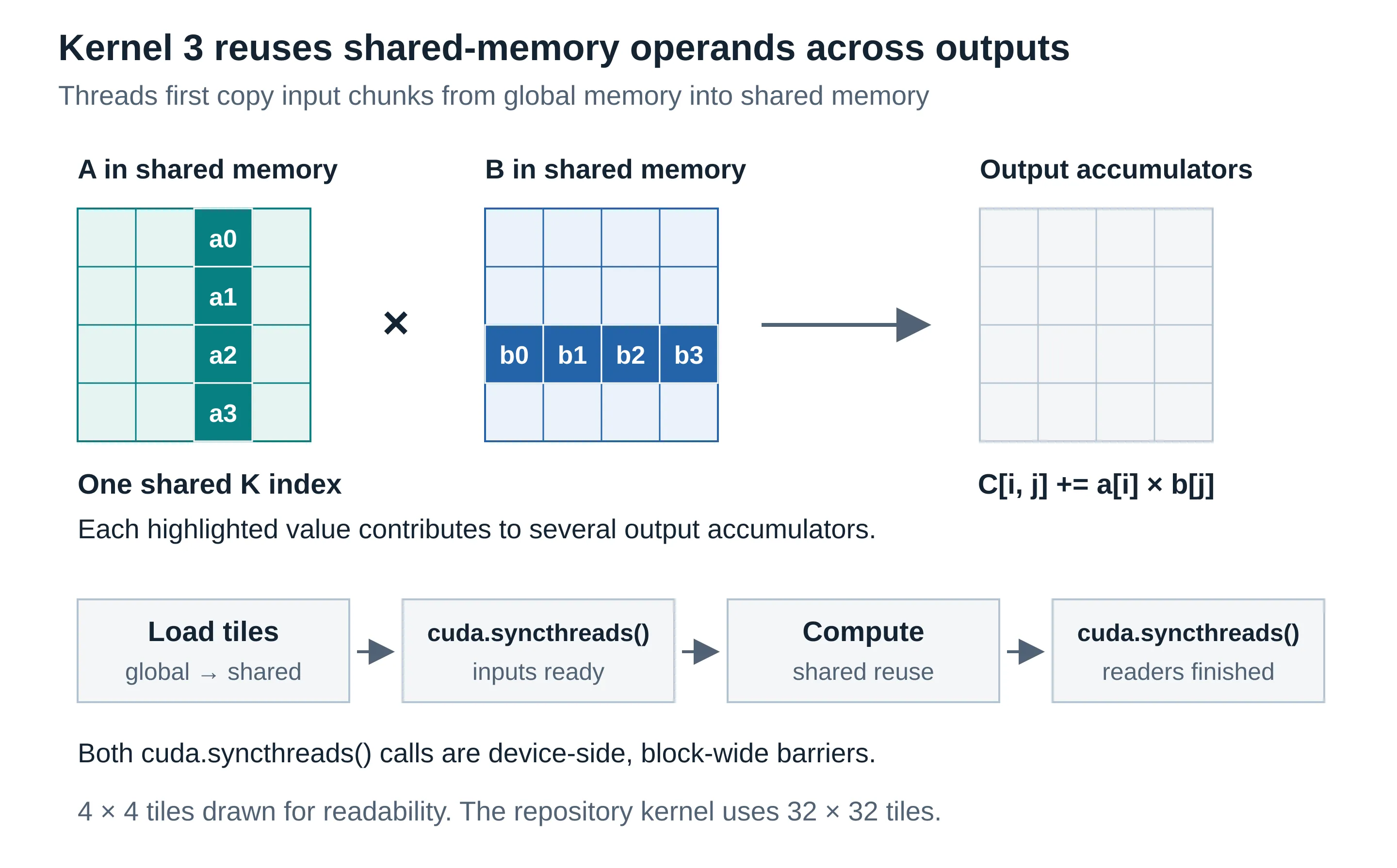
Kernel 3 introduced shared-memory tiles. Threads in a block cooperatively loaded portions of A and B, synchronized, and reused those values to compute a tile of C, so a value that contributed to several outputs no longer needed a separate global request for each use.

Consider a block computing a B_M × B_N tile of C from a chunk of B_K values along K. It needs an A panel of B_M × B_K values and a B panel of B_K × B_N values, and those panels support B_M × B_N × B_K multiply-adds. That reuse is what arithmetic intensity measures: operations performed per byte moved at a given memory level. For this simplified FP32 tile, ignoring output traffic, caches, and redundant loads:

Arithmetic intensity ≈ 2 B_M B_N B_K / [4 (B_M B_K + B_K B_N)] FLOP per byte

For a square B × B tile this simplifies to B/4 FLOP per byte of panel traffic. It’s a model, not a measurement, but it explains why reuse matters: the arithmetic grows faster than the panel traffic.

The cost was synchronization. Threads had to finish loading a shared tile before anyone consumed it, and could not overwrite it until the whole block was done reading. The tile created reuse, and it also created dependencies that later versions had to manage.

Kernel 4: several outputs per thread

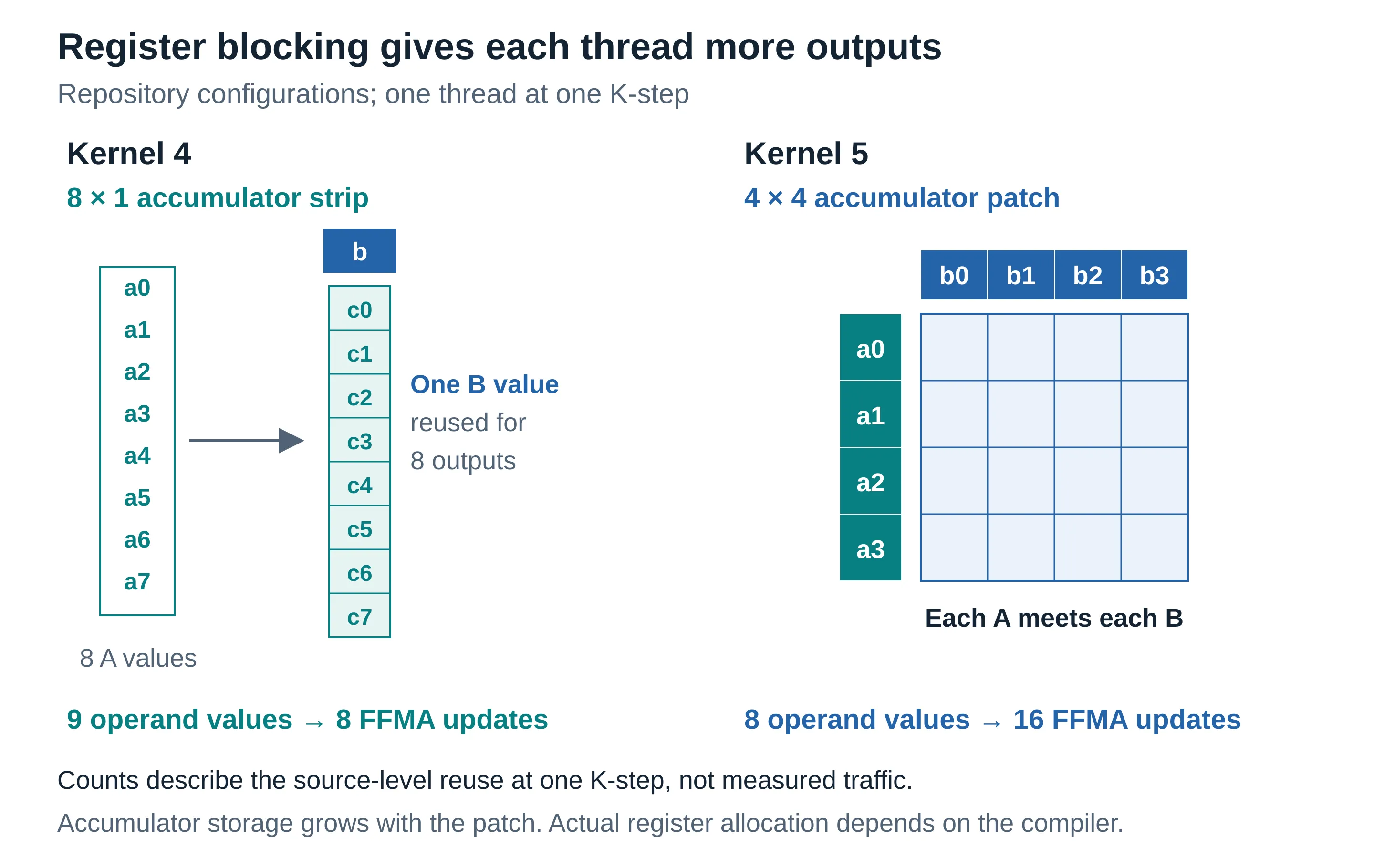
Kernel 4 moved more of that reuse into individual threads. Each thread kept a vertical strip of eight accumulators in registers, so one B value loaded per K-step fed eight multiply-adds with different A values. This is one-dimensional register blocking, and it made the resource trade visible: eight accumulators need more registers than one, and a change that reduces loads can still lose if its register demand leaves too little active work on the SM or causes spilling.

Kernel 5: reuse both operands in a register patch

Kernel 5 expanded the strip into a two-dimensional patch. The repository configuration used a 4 × 4 patch per thread inside a 64 × 64 block tile, with B_K = 16 and 256 threads. For a T_M × T_N patch, a thread loads T_M A values and T_N B values and uses their outer product to update T_M × T_N accumulators, so every A value is reused across T_N columns and every B value across T_M rows. The key change was not that the thread did more work, but that it did more multiply-adds per operand loaded into registers.

Block tiling and register blocking both increase reuse, at different levels. Block tiling cut repeated global requests by sharing panels among threads; register blocking cut repeated operand delivery to the arithmetic within a thread.

Kernel 6: organize the work at warp level

Kernel 6 added a level between the block tile and the thread patch: the block’s output tile was divided into warp-sized regions, and the 32 lanes of each warp covered their region together. It also stored A transposed in shared memory and expressed groups of four adjacent accesses, aligning the layout with the way threads consumed operands. (A source pattern that touches four adjacent values doesn’t prove the compiler emitted a vector load; the generated code has to be checked.)

The transpose matters because shared memory is split into 32 banks of four-byte words. Different addresses in the same bank force a warp’s access into extra service steps, so rearranging a shared tile can help even though the mathematics is unchanged. What counts is the set of addresses the lanes request for one instruction, not whether a drawing of the matrix looks contiguous. NVIDIA’s CUDA Best Practices Guide covers coalescing, shared-memory reuse, and bank conflicts.

Kernel 7: tune the geometry

Kernel 7 ran a Python autotuning search over 11 candidate configurations of block tile, warp tile, K-chunk depth, and thread patch. Numba compiled each candidate, and the harness timed them and kept the fastest. No single tile size wins by maximizing reuse alone: a larger tile reduces repeated loads but uses more registers or shared memory, a deeper K chunk reduces loop overhead but needs more buffering, and a warp arrangement that helps one operand’s access pattern can complicate the other’s. The search made those choices empirical.

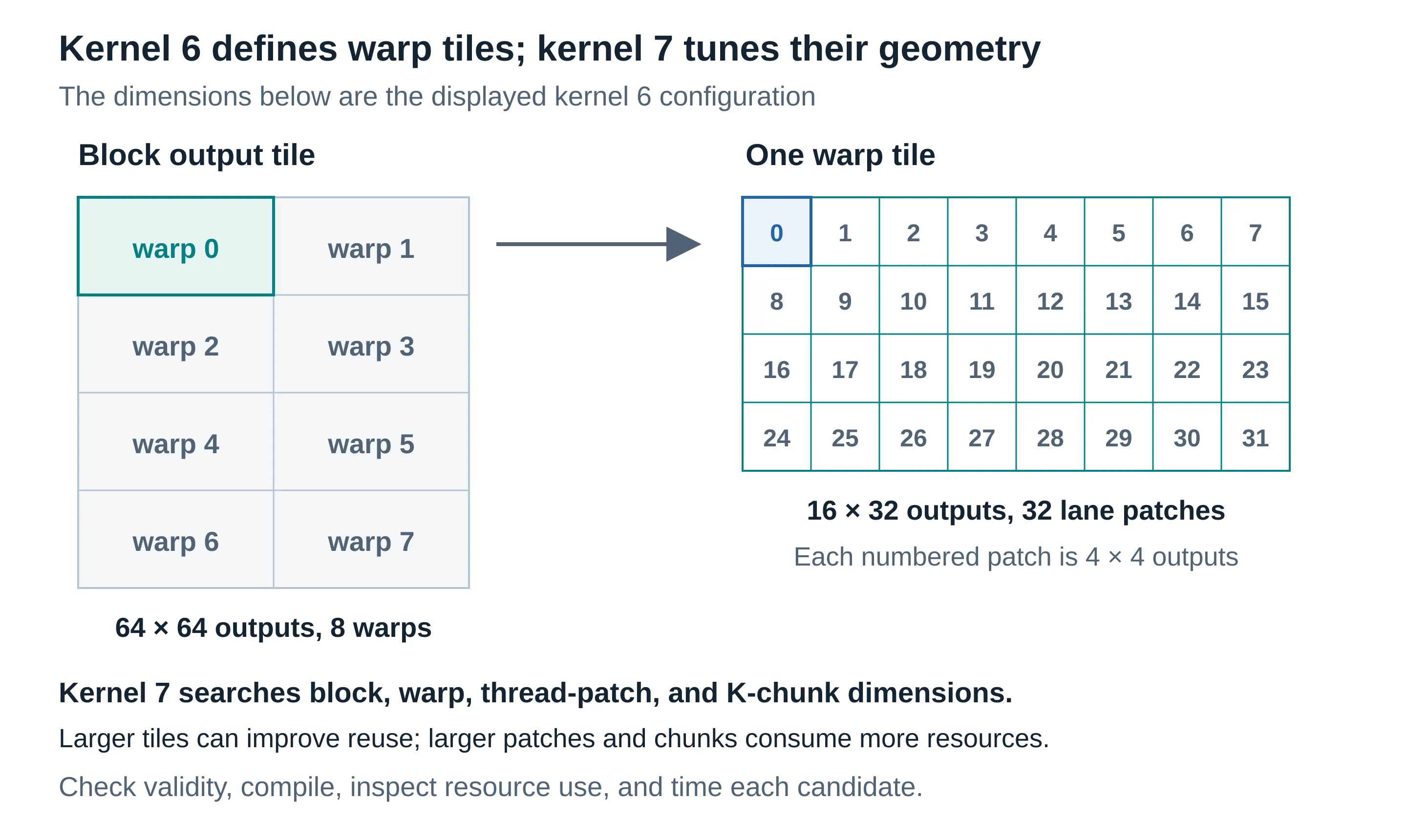
By this point the kernel had substantial data reuse. The remaining question was how consistently it could feed operands and instructions to the arithmetic units. If you want to watch kernels 1 to 7 step by step, the repository includes an interactive visualizer of each one’s thread ownership, global-memory sectors, shared-memory tiles, and registers:

Open the visualizer in its own tab (it needs a wide screen).

What the measurements can and can’t tell us

The starting point came from the course authors’ H100 measurements, not from my runs. The starting-point record in my lab notes preserves it: 86.6 µs for the course’s kernel 7 and 56.1 µs for cuBLAS at 1024 × 1024 FP32, about 65% of cuBLAS speed. I used those numbers as context for the challenge, not as a baseline. The record doesn’t capture the hardware model, software versions, clock policy, or repetition details, and the course’s measurement may have used different hardware or settings from mine. That likely accounts for its cuBLAS time (56.1 µs) being faster than the 64.6 µs cuBLAS measured in my confirmation run. So I never subtract my result from 86.6 µs and call the difference a speedup; every comparison below is against cuBLAS measured in the same run.

There is also an implementation boundary. Kernels 8 to 14 were written in CUDA C++ with inline PTX, compiled at runtime with NVRTC through CuPy’s RawKernel, with separate nvcc builds for inspecting SASS (the GPU’s machine instructions). That is not a sequence of edits to the Numba kernel under the same compiler, so any comparison across the boundary includes changes in code generation as well as in the optimization itself.

The investigation used timings and profiles for different jobs. Timings decided whether a candidate was useful. Nsight Compute, including its per-instruction source view, suggested where to look next. A proposed explanation stayed a hypothesis until the code and the timings supported it. A counter comparison at one fixed configuration and the fastest result from a configuration sweep also answer different questions, and I’ve tried to say which one each number is.

Kernel 8: asynchronous copies

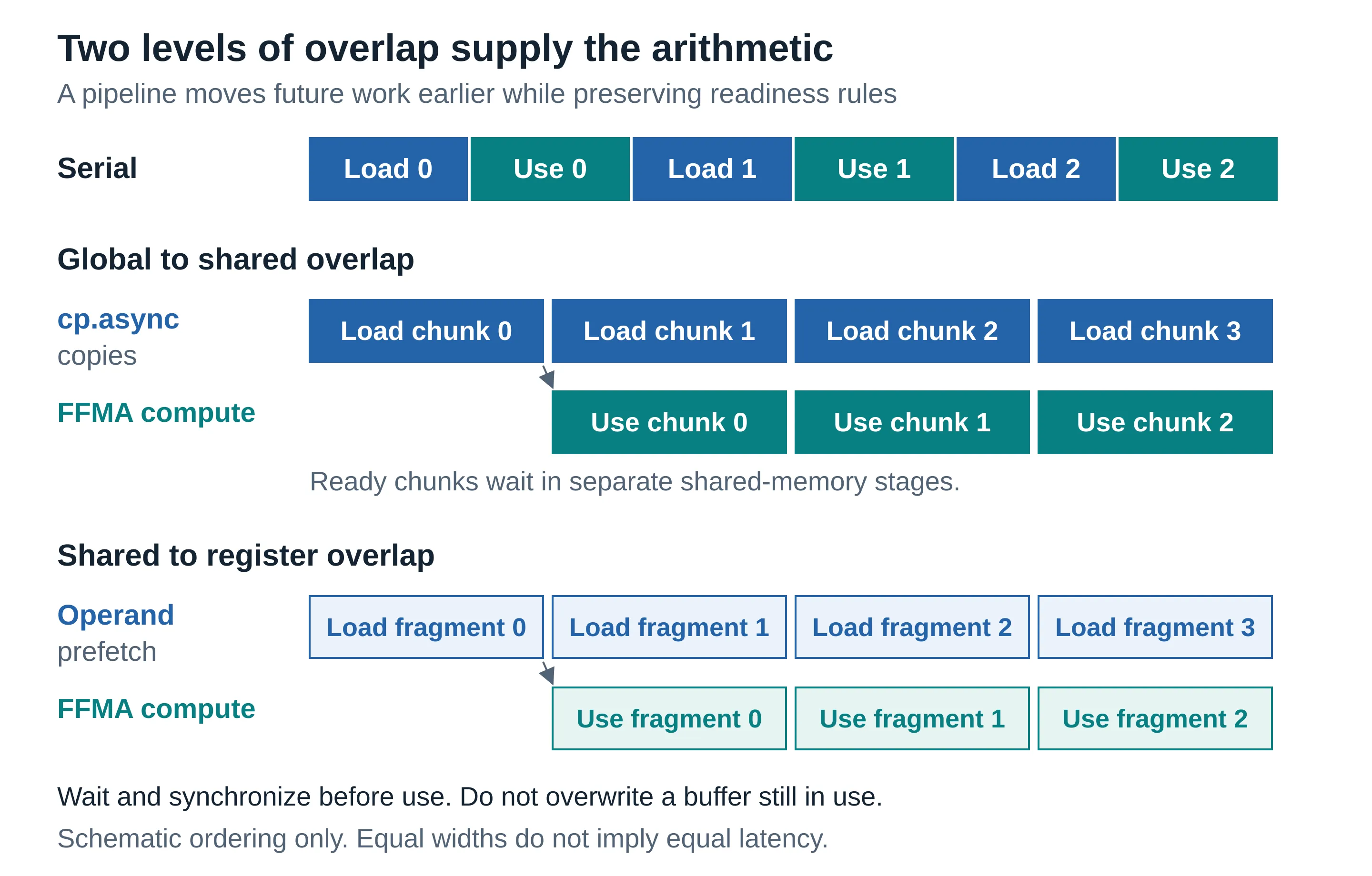
A GEMM kernel repeatedly loads chunks along the shared K dimension. In a simple implementation the block loads a chunk, waits until it’s usable, does the arithmetic, and then moves on, which is the load, synchronize, compute cycle in Figure 4. During those waits the arithmetic units may have nothing to issue from that warp.

Kernel 8 introduced per-thread cp.async copies from global memory into a multi-stage shared-memory ring buffer: a fixed set of reusable buffers, called stages, visited in a repeating order (with three stages: 0, 1, 2, then back to 0). Each stage holds one K chunk. The pipeline loads a future chunk into one stage while computing on a ready chunk in another, and reuses a stage only after its previous contents are no longer needed.

The cp.async primitives issue an asynchronous global-to-shared copy, and issuing a copy is not the same as having its result. cp.async.wait_group waits on the issuing thread’s own copy groups, and __syncthreads() then makes every thread’s copies visible across the block: copy completion and coordination between threads are separate requirements. The benefit is a chance to put useful arithmetic between issuing a request and waiting for it, instead of stopping after every load. NVIDIA’s asynchronous copy documentation describes the model.

More stages aren’t free: they occupy shared memory, and if buffering reduces the number of blocks that fit on an SM the trade can go the wrong way. So stage count went into the configuration search.

At the fixed configuration used for the profile (128 × 64 tiles, B_K = 8, n = 1,024), the share of warp cycles spent waiting on global memory (Nsight’s long-scoreboard stall) fell from 46.8% with one stage to 2.5% with three, below cuBLAS’s 6.6%. The best 1,024 configuration in that sweep reached about 89% of cuBLAS. The single-stage control was not identical to the course’s kernel 7, so this doesn’t isolate the full difference between the course implementation and this one. The remaining gap was in how often the scheduler issued instructions, not in memory.

This was ordinary per-thread cp.async. TMA, the Hopper Tensor Memory Accelerator, appears later only as a proposed experiment; it is not part of any measured result.

Kernel 9: the next operand bottleneck

Kernels 8 and 9 apply the same idea at two levels of the hierarchy: prepare future operands while computing with ones that are already ready. Kernel 8 pipelined global-to-shared copies. Kernel 9 kept that pipeline and added shared-to-register prefetching into two alternating sets of registers. One set holds the operands for the current K-step while ordinary shared-memory loads fill the other for the next step (no second cp.async path is involved). That doesn’t make a dependent multiply-add independent of its inputs; it moves the load earlier, so the inputs are more likely to be ready when the multiply-add needs them.

A separate switch stored A transposed in shared memory, so a thread’s eight A values for a K-step could be fetched with two 128-bit (float4) loads instead of eight scalar loads. As with kernel 6, the generated instructions are what count: a source expression that mentions four values isn’t proof of one vector load.

Two Nsight metrics were useful here because they describe different halves of the hypothesis. The short-scoreboard stall tracks a class of dependency waits that includes shared-memory results; it is not “all time spent loading shared memory.” Issue-active is how often the scheduler issued an instruction; it is not a percentage of peak FLOP/s. The Nsight Compute Profiling Guide is the reference for both. With both changes, short-scoreboard stalls fell from 0.38 to 0.13 cycles per issued instruction and issue-active rose from 52% to 62%. The best 1,024 configuration reached about 97% of cuBLAS.

The two switches were also measured separately, and alone each gave mixed results:

Timing sweep

128×64 tile, BK16, 3 stages · cuBLAS 65.3 µs

no prefetchprefetch

A row-major73.9 µskernel 874.6 µs+1% slower

A transposed71.1 µs−4% faster67.6 µs−9% faster

Nsight Compute profile

128×64 tile, BK8, 3 stages · cuBLAS 61.3 µs

no prefetchprefetch

A row-major78.4 µskernel 877.4 µs−1% faster

A transposed89.2 µs+14% slower71.5 µs−9% faster

Show the data

Measurement	Variant	Time (µs)
Timing sweep	kernel 8 (neither)	73.9
Timing sweep	transposed A only	71.1
Timing sweep	register prefetch only	74.6
Timing sweep	both (kernel 9 + T)	67.6
Nsight Compute profile	kernel 8 (neither)	78.4
Nsight Compute profile	transposed A only	89.2
Nsight Compute profile	register prefetch only	77.4
Nsight Compute profile	both (kernel 9 + T)	71.5

The consistent result was the combination. Without prefetch, the transposed layout’s wider loads still stalled the warp that issued them; without the transpose, prefetch needed eight scalar loads per fragment. Together, the loads could move earlier and there were fewer of them. That win was limited to n = 1,024: at 2,048 and 4,096, kernel 9 gave no gain (79–83% of cuBLAS).

A plausible optimization that didn’t improve runtime

The larger matrices suggested another opportunity. At n = 4,096 each matrix is 64 MB, more than the H100’s 50 MB L2 cache, and blocks launched in plain row order. Changing the order in which blocks process output tiles (block swizzling) can make neighboring blocks reuse more of the same input panels through L2, and if fewer bytes reach DRAM it’s reasonable to expect the kernel to get faster. I grouped launches eight block-rows at a time, similar to Triton’s GROUP_M.

The swizzle did what it was designed to do. DRAM reads fell by 22% and 53% on the two configurations tested, and the L2 hit rate rose. Runtime didn’t follow:

k9, 128×128 tilek9 + transposed A, 128×64 tilecuBLAS

Show the data

Kernel	Launch order	DRAM read (MB)	ncu time (ms)
k9, 128×128 tile	row order	595.6	3.058
k9, 128×128 tile	swizzled	462.6	3.475
k9 + transposed A, 128×64 tile	row order	962.5	3.464
k9 + transposed A, 128×64 tile	swizzled	454.7	3.340
cuBLAS	—	342.3	2.647

The profile explains why. Time spent waiting on global memory was at most 6% in every case, swizzled or not. At n = 4,096 the best later kernel needs about 0.13 TB/s of HBM bandwidth, roughly 4% of what the H100 provides. DRAM traffic was not what limited these kernels, so cutting it changed nothing that mattered. This is the clearest example of a successful local change that wasn’t a performance improvement, and it would have been easy to keep the change on the strength of the memory counters alone. (The switch stayed on in later kernels because it didn’t hurt.)

Larger thread patches and less address bookkeeping

Kernel 10: bigger patches

Kernel 10 increased the per-thread patch to 16 × 8 or 8 × 16, the same 128 outputs per thread that cuBLAS’s own kernel uses at n = 4,096. A T_M × T_N outer product uses T_M + T_N operand values to update T_M × T_N accumulators, so larger patches make each operand serve more multiply-adds. But accumulator count grows with the product of the dimensions, and these configurations ran at about 255 registers per thread.

The layout had to change with the patch. With eight thread columns, contiguous B columns would put two lanes in the same shared-memory bank, a two-way conflict, so kernel 10 used a strided mapping for B columns that is conflict-free. Both the amount of work per thread and the way threads fetched operands changed, so “a larger tile” isn’t a complete explanation of the result.

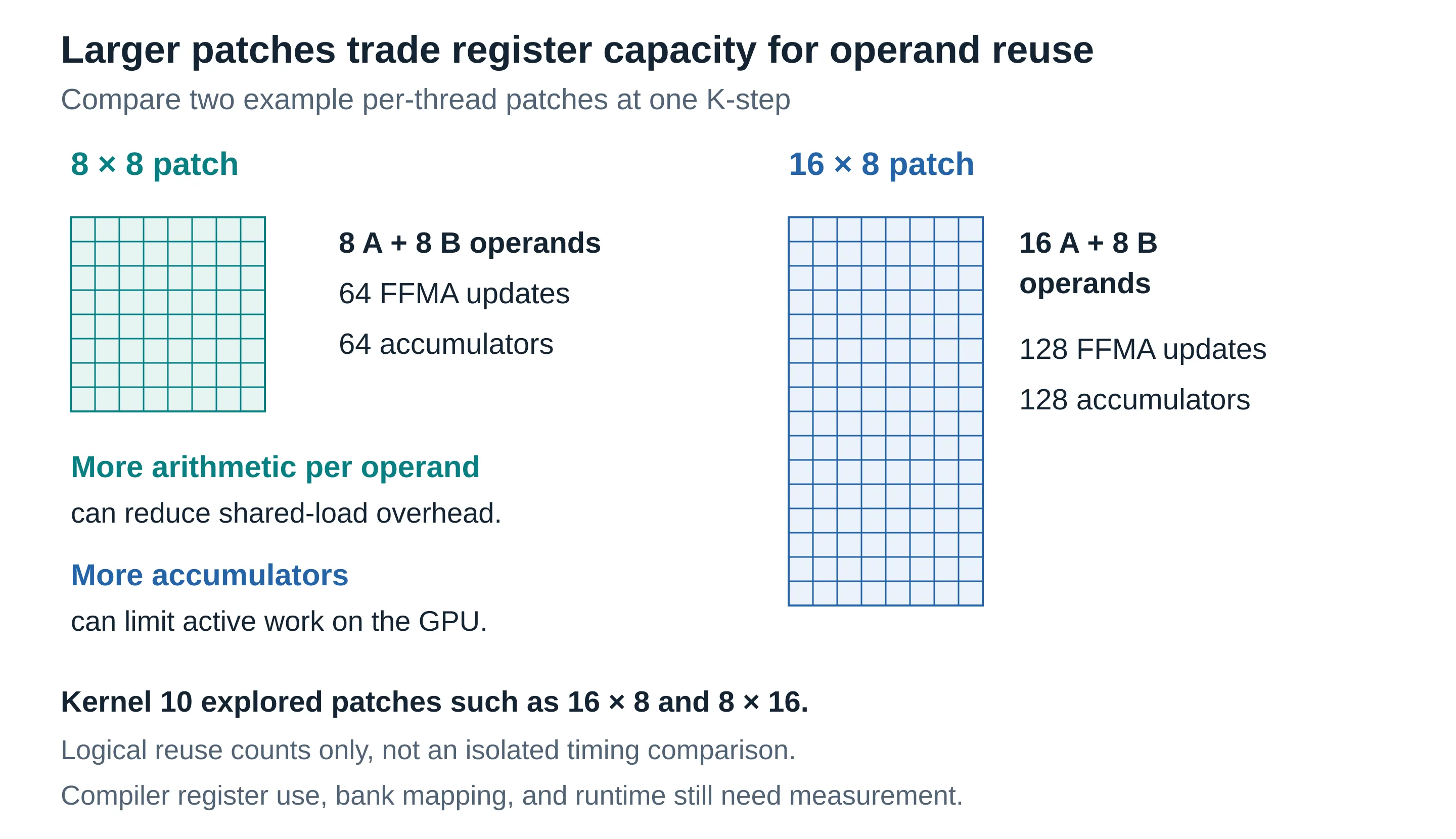
At n = 4,096, shared-memory loads fell from 336 million to 101 million, matching cuBLAS, and performance reached about 90% of cuBLAS (88% at 2,048). The n = 1,024 result dipped at this step, from 97% to 92%, but that dip was on the same 128 × 64 configuration as before, not on the new large patches. It coincided with the B-column remap, a later test (kernel 13) ruled the remap out, and I never isolated the cause, so I treat it as likely run-to-run variation rather than a property of larger patches.

Kernel 11: hoist the address math

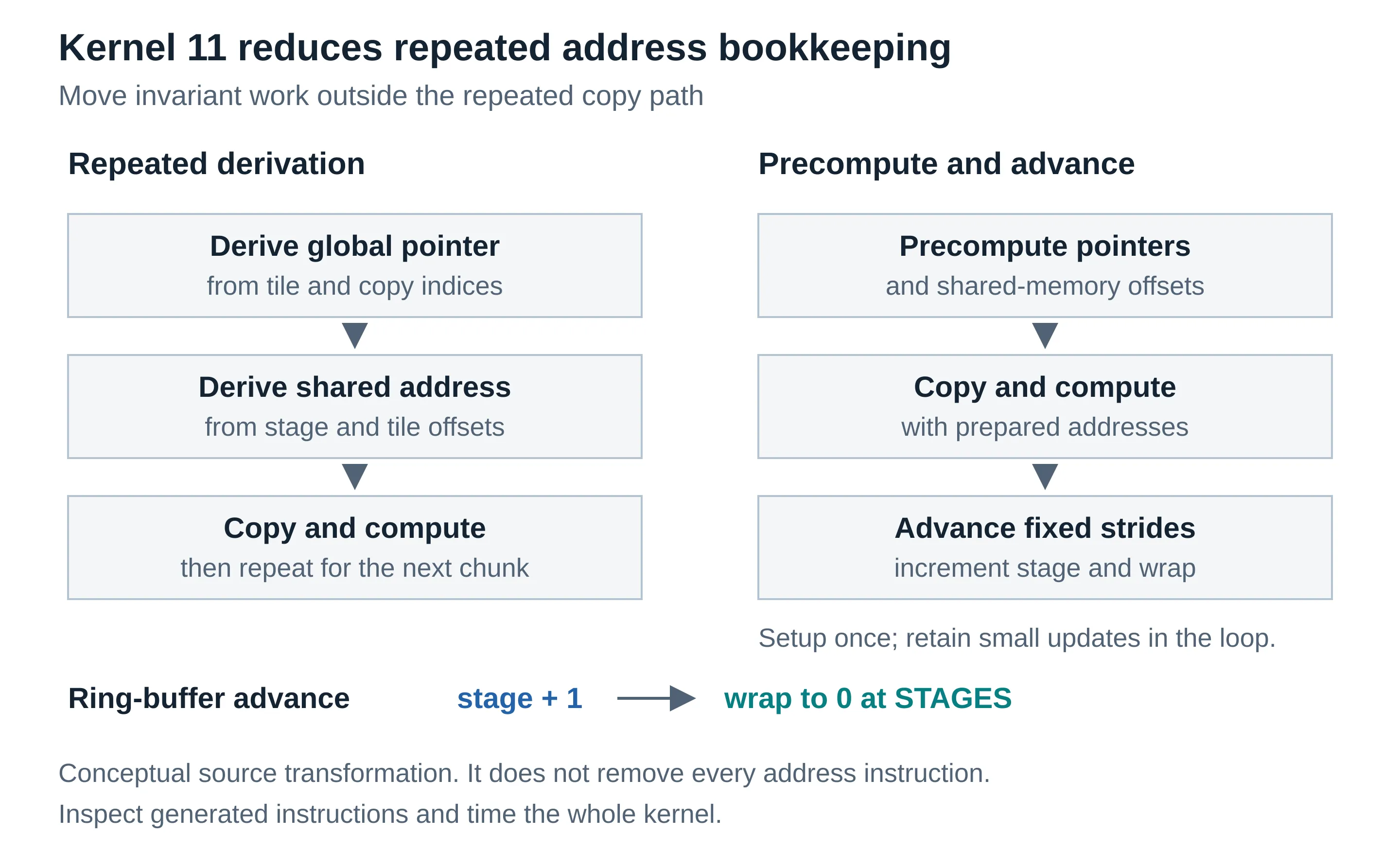
At this point, Nsight’s per-instruction view showed the hot loop spending a lot of issue slots on integer instructions (LEA, IMAD, LDC) that cuBLAS’s hot loop didn’t execute at all. At 255 registers, the compiler was re-reading the matrix dimensions from constant memory and recomputing every cp.async source address for every chunk. Kernel 11 precomputed each thread’s copy pointers and shared-memory offsets once (hoisting them out of the loop), advanced them by fixed strides, and replaced the ring buffer’s t % STAGES with add-and-wrap. None of this reduces the multiply-adds the product needs; it reduces the work around them.

Overhead instructions per FFMA fell from 0.170 to 0.075 (cuBLAS: 0.131), registers dropped from 255 to 231, and the larger sizes reached 94–95% of cuBLAS. Not every prediction held: wait stalls fell to 0.08 rather than the predicted 0.02, and the per-instruction view showed why. The running pointer update had compiled into a chain of dependent 64-bit multiply-adds issued in one burst at each chunk boundary.

Loop unrolling supported several of these changes. The CUDA C++ file unrolls every loop with a compile-time trip count, which is what lets the accumulators and double buffers live in registers and turns kernel 11’s offsets into instruction immediates (CUDA C++ loop-unrolling controls). The course’s Numba kernels already unrolled their small inner patch loops but not the K-step loop. I never measured unrolling on its own, and comparisons of instruction counts across different configurations and GPUs can’t assign a gain to it alone.

Kernels 12 and 13: refine the schedule without adding overhead

Kernel 11’s remaining stalls clustered at chunk boundaries, so kernel 12 spread each chunk’s copies across the K-steps, addressing each from the chunk’s base so there was no dependency chain, and separately tried a different multiply-add order. Two versions can move the same bytes and perform the same arithmetic but expose very different dependency chains to the scheduler. Issuing a load earlier helps if independent instructions are available before its result is needed; it doesn’t help if the change adds enough bookkeeping to consume the time it saved.

Kernel 12 showed both sides. In its own sweep it reached parity with cuBLAS at n = 1,024 (64.9 µs against 64.8, a tie within run-to-run noise, with the alternate FFMA order) and was the best kernel yet at 2,048 (355.6 µs against 340.9, 96%). At 4,096 it gained nothing: 2,779.4 µs against kernel 11’s 2,772.9. The stalls it targeted did fall, but it executed about 57 million more instructions, and the breakdown wasn’t the address arithmetic I’d expected:

Show the data

Instruction group	SASS	Extra instructions executed
Filler shared loads	@!PT LDS RZ, [RZ]	+25.203 M
Register moves	MOV R, URx	+15.688 M
Kernel-parameter reloads	ULDC	+10.490 M
All other opcodes (net)	UISETP, PLOP3, LEA, …	+5.693 M
Total		+57.074 M (2,322 M → 2,379 M)

LDS is a shared-memory load; the @!PT predicate is never true, so the instruction does nothing, but it still occupies an issue slot. MOV moves values between registers, and ULDC loads a constant through the uniform datapath. The likely source of both is the per-K-step branch that decided whether to issue a spread copy, though I didn’t prove that. Either way, a better stall counter wasn’t evidence of a faster kernel; the runtime decided.

Kernel 13 tested three things. A branch-free version of copy spreading, which always issues every copy and uses a zero-byte copy past the end, didn’t buy time. Reverting to contiguous B columns, to test whether kernel 10’s remap had hurt, was worse everywhere, by up to 10% at n = 4,096: the useful layout was the one that suited the warp’s actual accesses, not the one that looked simplest. And size specialization, compiling the matrix size in as a constant so the compiler can fold address math into immediates, gave about one point at large sizes. A specialized kernel is a legitimate candidate for a fixed workload, but it doesn’t have the flexibility of a library routine that accepts sizes at runtime, so the results report specialized and generic candidates separately.

Kernel 14 and Stream-K

At n = 1,024, every kernel so far, cuBLAS included, ran one warp per scheduler. The best configuration (kernel 11, 128 × 64 tiles) launched 128 blocks of four warps onto 132 SMs: at most one block per SM, so each of an SM’s four warp schedulers had exactly one warp to choose from. When that warp stalled on a dependency, the scheduler had nothing else to issue, which is why short-scoreboard and dispatch stalls showed up directly as lost issue slots. Making each individual operation faster doesn’t fix that; the scheduler needs a second warp.

Kernel 14 returned to the hoisted kernel 11 design and added a persistent Stream-K kernel. It’s a branch from kernel 11, not kernel 13 with every experiment retained; the variant definitions show the winning variant uses neither copy spreading nor size specialization. A persistent kernel launches only as many blocks as fit at once (264 here, two per SM) and loops over the work. Stream-K changes the unit of that work: instead of each block owning one output tile’s entire K reduction, the stream of (tile, K-chunk) steps is divided evenly across blocks, so a block boundary can fall partway through a tile. This implementation does full waves of whole tiles first and splits only what’s left. At n = 1,024 with 128 × 128 tiles there are just 64 tiles, fewer than the 264 resident blocks, so all of the work is split, and each tile’s K range is shared by roughly four blocks. Their partial sums are combined with vector atomicAdd into an output that a separate kernel zeroes first.

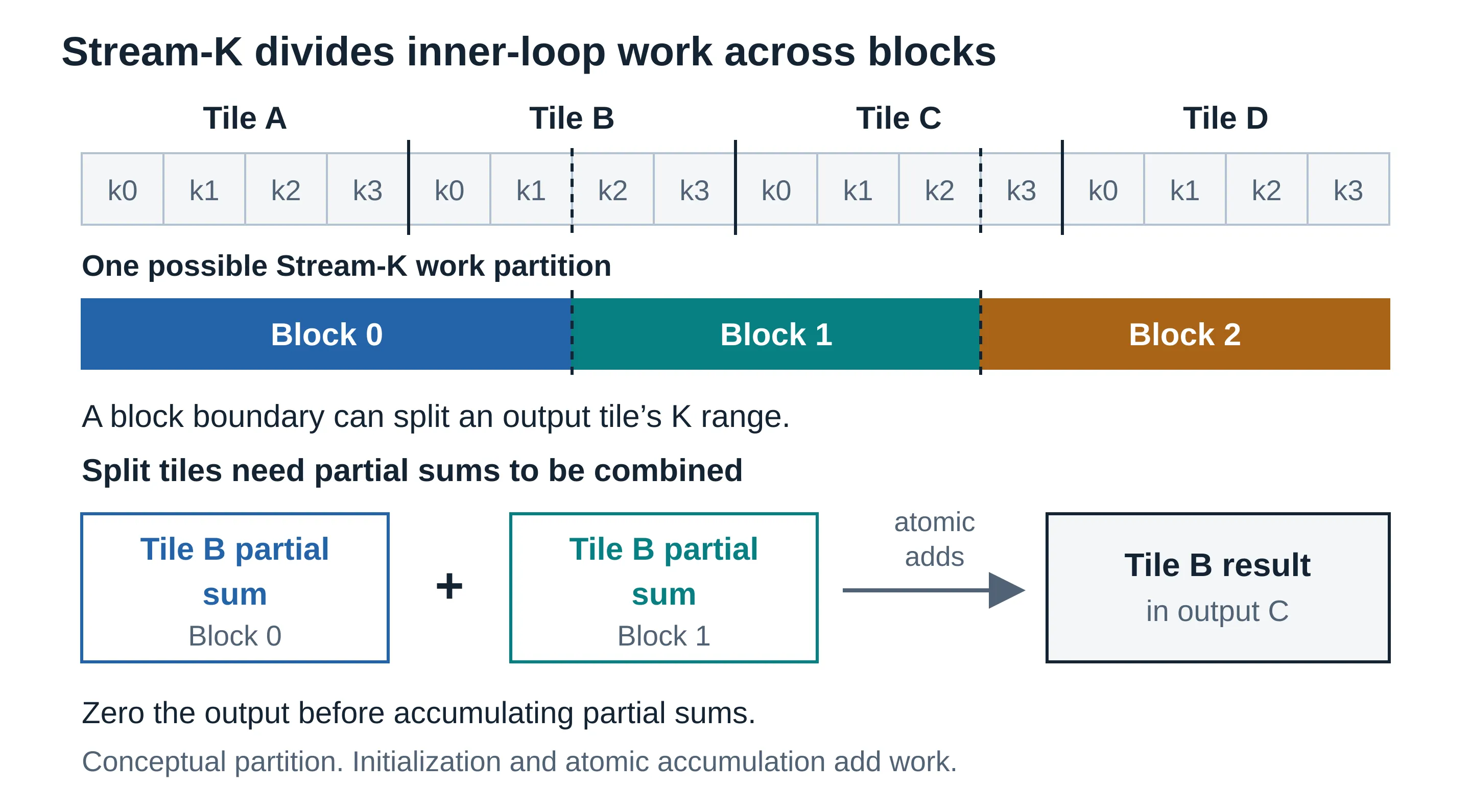
This didn’t make the matrix multiplication smaller. It redistributed the work so each scheduler had two warps, and it added work of its own: zeroing the output, the atomic accumulation, and a different summation order. The profile shows what that bought:

k11 128×64 (best before Stream-K)k14 128×128 (Stream-K)cuBLAS

Show the data

Kernel (ncu, n = 1,024)	Warps per scheduler	Issue active	Stall cycles per issued instr.
k11 128×64 (best before Stream-K)	1.00	62.6%	1.60
k14 128×128 (Stream-K)	1.99	72.0%	2.77
cuBLAS	1.00	69.9%	1.43

The counterintuitive part is the third panel. The win didn’t come from any warp stalling less; per-warp stalls went up. It came from having a second warp to cover them. The confirmation timing included both the zeroing kernel and the Stream-K kernel, because a result that counted only the fast part of the computation would be much less useful.

The confirmed result

The final confirmation ran on an NVIDIA H100 80GB HBM3 (132 SMs) on Modal, with CUDA 13, PyTorch 2.14.1+cu130, and CuPy 14.2. The cuBLAS reference was torch.matmul, with FP32 inputs and arithmetic and TF32 disabled. Each candidate was checked for correctness first. cuBLAS and the candidates were then timed in 15 alternating rounds, each reporting the median of 40 CUDA-event measurements, with a 256 MiB buffer written before each launch to flush L2. Comparing each kernel against cuBLAS within the same round cancels slow drift in clocks and temperature. Those conditions matter when comparing these numbers with benchmarks that reuse warm data.

At 1024 × 1024, the generic kernel 14 configuration took 61.328 µs against 64.624 µs for cuBLAS. The median paired speed ratio was 1.05295 (105.0–105.8% across rounds), and the custom kernel was ahead in all 15 rounds. That’s about 5.3% higher throughput, or 5.1% lower latency. At 2048 × 2048, the best size-specialized kernel 13f took 357.9 µs against 341.3 µs, 95.4% of cuBLAS; at 4096 × 4096 it took 2,761.2 µs against 2,661.1 µs, 96.4%. The best generic kernel 11 configurations reached 93.9% and 95.2% at those sizes. The best numbers across sizes didn’t all come from one universally winning kernel.

In absolute terms, kernel 14 at n = 1,024 ran at 35.0 TFLOP/s against cuBLAS’s 33.2, which is 57% and 54% of the 61.3 TFLOP/s FP32 FFMA ceiling I measured on an H100 in an earlier course assignment. At n = 4,096, k13f reached 49.8 TFLOP/s against cuBLAS’s 51.6 (81% and 84%). “Beating cuBLAS” here means getting closer to the same compute roof than cuBLAS did at one size, not exceeding the hardware.

k14 (Stream-K)k11 (generic)cuBLASMeasured roof

Show the data

Size	Kernel	AI (FLOP/byte)	TFLOP/s	% of 61.3 TFLOP/s
n = 1,024	k14 Stream-K	≈ 170	35.0	57%
n = 1,024	cuBLAS	≈ 170	33.2	54%
n = 1,024	k11	≈ 170	32.5	53%
n = 4,096	cuBLAS	≈ 338	51.6	84%
n = 4,096	k11 128×256	≈ 314	49.2	80%

That picture summarizes the whole investigation. None of the kernels was limited by DRAM bandwidth, so the swizzle’s traffic reduction had nowhere to go. Every gain from kernel 8 to kernel 14 moved a point straight up toward the roof by raising issue efficiency: hiding latency (kernels 8 and 9), executing fewer overhead instructions (10 and 11), and giving each scheduler more warps (14).

What the result establishes

The 1,024 result is a repeatable win within the tested setup, with a limited scope. The experiments covered square, tile-multiple shapes, not arbitrary dimensions with edge handling. Stream-K’s atomic accumulation changes summation order, so results are not bit-reproducible. Correctness was checked by requiring finite outputs and a maximum absolute error, normalized by the reference’s maximum absolute value, below 10⁻⁴.

The remaining gap at larger sizes gives a concrete next question. Stream-K helped the small case, but the measured Stream-K variants lost to the non-Stream-K kernels at 2,048 and 4,096 (89–94%). Higher register use from inlining the tile body twice is a plausible contributor, not an isolated cause. TMA is another proposed direction, starting with B’s copies while preserving A’s working layout. Neither should be described as a measured success yet.

Summary

The useful progression in this work was the sequence of questions. After improving reuse, I checked whether global-memory latency was exposed. After overlapping those copies, I looked at shared-memory operand delivery. After increasing arithmetic per load, I looked at the address instructions around that arithmetic. And for the small case, the final improvement came from giving each scheduler more than one warp.

The first seven kernels had already fixed inefficient global accesses and established reuse through shared-memory tiles, register patches, and warp-level organization. The later experiments didn’t discard that foundation; they investigated what still prevented it from supplying the arithmetic consistently. Async copies reduced exposed global-memory waiting. Register double buffering and the transposed layout targeted the next operand dependency, and only worked together. Larger patches cut shared-load work, and hoisting cut the instructions around the multiply-adds. The swizzle and copy-spreading experiments showed why a better-looking counter didn’t always mean a better runtime. Stream-K provided enough parallel work to produce a repeatable win at 1,024.

That sequence is also where the LLM-assisted process needs scrutiny. A plausible explanation can point to a useful experiment, but the explanation alone doesn’t establish what made the kernel faster. The source, the generated instructions, the correctness checks, and the timings are what let me decide which parts of the story hold up.

Evidence for review

Course information is on the workshop website and the Maven course page; Vizuara AI Labs is the organization’s main site. The official course repository has the course source. The course credits Simon Boehm’s worklog as an inspiration; the explanations here follow the course repository, with the worklog as an external comparison.

My fork holds the lab implementations and the later experiments. Every link in this article is pinned to that commit, so the line numbers won’t drift:

• Kernels 1–4: Lecture8_MatMul_Kernels.ipynb
• Kernels 5–7: matmul-05.py, matmul-06.py, matmul-07.py
• Kernels 8–14 share matmul_cp_async.cu, with build switches and the variant mapping in matmul08.py
• The investigation narrative: LAB_NOTEBOOK.md and BIG_WINS.md
• The final confirmation: machine-readable JSON and a readable summary
• The interactive visualizer: visualizations/kernels

The confirmation artifacts date to November 4, 2026, and include source snapshots whose SHA-256 hashes match the linked source. Early profiler evidence is less complete because some profiles were overwritten; the results manifest distinguishes surviving and rebuilt records. The performance claims above use confirmation timings, not Nsight replay timings; the charts of profiler counters say so where they’re used.

The early lab files are learning artifacts, not production-ready implementations. In particular, the saved kernel 5 and 6 files accumulate into local arrays without an explicit zero-initialization loop, which needs review before using them as standalone examples, and the final correctness checks apply to the later candidates, not retroactively to every early lab file. The kernel 1 and 2 explanations follow the executable index expressions; the notebook’s opening coalescing comments don’t consistently match them.